This page was generated from source/notebooks/L5/numpy/1-Exploring-data-using-numpy.ipynb.

Exploring data using NumPy

Our first task in this week’s lesson is to learn how to read and explore data files using NumPy. Reading data files using NumPy will make life a bit easier compared to the traditional Python way of reading data files. If you’re curious about that, you can check out some of the lesson materials from past years about reading data in the Pythonic way.

What is NumPy?

NumPy is a library for Python designed for efficient scientific (numerical) computing. It is an essential library in Python that is used under the hood in many other modules (including Pandas). Here, we will get a sense of a few things NumPy can do.

Preparation (the key to success)

Presumably you have already opened this Jupyter notebook (if not, do so now using one of the links above), and our first task is to change the working directory to the one containing the files for this week’s lesson (in this case the numpy directory. You can do that by first checking which directory Jupyter is operating in using the %ls IPython magic command.

%ls

If you see files like 1-Exploring-data-using-numpy.ipynb, you’re all set. If not, you can change the working directory using the %cd magic command. For example,

%cd L5/numpy/

[Errno 2] No such file or directory: 'L5/numpy/'
/Users/whipp/Work/Teaching-and-seminars/HY/Geo-Python/Fall-2018-git/source/notebooks/L5/numpy

The command above gives an error in this case because we’re in a different directory, but you get the point. If you need some additional help to get into the right working directory, you can refer back to the lesson on functions where we covered changing the working directory in more detail.

Reading a data file with NumPy

Importing NumPy

Now we’re ready to read in our temperature data file. First, we need to import the NumPy module.

import numpy as np

That’s it! NumPy is now ready to use. Notice that we have imported the NumPy module with the name np.

Reading a data file

Now we’ll read the file data into a variable called data. We can start by defining the location (filepath) of the data file in the variable fp.

fp = '../Kumpula-June-2016-w-metadata.txt'

Now we can read the file using the NumPy genfromtxt() function.

data = np.genfromtxt(fp)

np.genfromtxt() is a general function for reading data files separated by commas, spaces, or other common separators. For a full list of parameters for this function, please refer to the NumPy documentation for numpy.genfromtxt().

Here we use the function simply by giving the filename as an input parameter. If all goes as planned, you should now have a new variable defined as data in memory that contains the contents of the data file. You can check the the contents of this variable by typing the following:

print(data)

[nan nan nan nan nan nan nan nan nan nan nan nan nan nan nan nan nan nan
 nan nan nan nan nan nan nan nan nan nan nan nan nan]

Inspecting our data file

Hmm…something doesn’t look right here. You were perhaps expecting some temperature data, right? Instead we have only a list of nan values.

nan stands for “not a number”, and might indicate some problem with reading in the contents of the file. Looks like we need to investigate this further.

We can begin our investigation by opening the data file in JupyterLab by right-clicking on the Kumpula-June-2016-w-metadata.txt data file and selecting Open.

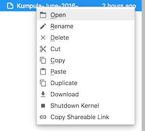
You should see something like the following:

# Data file contents: Daily temperatures (mean, min, max) for Kumpula, Helsinki # for June 1-30, 2016 # Data source: https://www.ncdc.noaa.gov/cdo-web/search?datasetid=GHCND # Data processing: Extracted temperatures from raw data file, converted to # comma-separated format # # David Whipp - 02.10.2017 YEARMODA,TEMP,MAX,MIN 20160601,65.5,73.6,54.7 20160602,65.8,80.8,55.0 ...

We can observe a few important things:

• There are some metadata at the top of the file (a header) that provide basic information about its contents and source. This isn’t data we want to process, so we need to skip over that part of the file when we load it.
  • We can skip the top header lines in the file using the skip_header parameter.
• The values in the data file are separated by commas.
  • We can specify the value separator using the delimiter parameter.
• The top row of values below the header contains names of the column variables.
  • We’ll deal with those later.

Reading our data file, round 2

Let’s try reading again with this information in mind.

data = np.genfromtxt(fp, skip_header=9, delimiter=',')

Note that we now skip the header lines (first 9 lines) using skip_header=9 and tell NumPy the files is comma-separated using delimiter=','.

Let’s print out the contents of data now and see how things look.

print(data)

[[2.0160601e+07 6.5500000e+01 7.3600000e+01 5.4700000e+01]
 [2.0160602e+07 6.5800000e+01 8.0800000e+01 5.5000000e+01]
 [2.0160603e+07 6.8400000e+01 7.7900000e+01 5.5600000e+01]
 [2.0160604e+07 5.7500000e+01 7.0900000e+01 4.7300000e+01]
 [2.0160605e+07 5.1400000e+01 5.8300000e+01 4.3200000e+01]
 [2.0160606e+07 5.2200000e+01 5.9700000e+01 4.2800000e+01]
 [2.0160607e+07 5.6900000e+01 6.5100000e+01 4.5900000e+01]
 [2.0160608e+07 5.4200000e+01 6.0400000e+01 4.7500000e+01]
 [2.0160609e+07 4.9400000e+01 5.4100000e+01 4.5700000e+01]
 [2.0160610e+07 4.9500000e+01 5.5900000e+01 4.3000000e+01]
 [2.0160611e+07 5.4000000e+01 6.2100000e+01 4.1700000e+01]
 [2.0160612e+07 5.5400000e+01 6.4200000e+01 4.6000000e+01]
 [2.0160613e+07 5.8300000e+01 6.8200000e+01 4.7300000e+01]
 [2.0160614e+07 5.9700000e+01 6.7800000e+01 4.7800000e+01]
 [2.0160615e+07 6.3400000e+01 7.0300000e+01 4.9300000e+01]
 [2.0160616e+07 5.7800000e+01 6.7500000e+01 5.5600000e+01]
 [2.0160617e+07 6.0400000e+01 7.0700000e+01 5.5900000e+01]
 [2.0160618e+07 5.7300000e+01 6.2800000e+01 5.4000000e+01]
 [2.0160619e+07 5.6300000e+01 5.9200000e+01 5.4100000e+01]
 [2.0160620e+07 5.9300000e+01 6.9100000e+01 5.2200000e+01]
 [2.0160621e+07 6.2600000e+01 7.1400000e+01 5.0400000e+01]
 [2.0160622e+07 6.1700000e+01 7.0200000e+01 5.5400000e+01]
 [2.0160623e+07 6.0900000e+01 6.7100000e+01 5.4900000e+01]
 [2.0160624e+07 6.1100000e+01 6.8900000e+01 5.6700000e+01]
 [2.0160625e+07 6.5700000e+01 7.5400000e+01 5.7900000e+01]
 [2.0160626e+07 6.9600000e+01 7.7700000e+01 6.0300000e+01]
 [2.0160627e+07 6.0700000e+01 7.0000000e+01 5.7600000e+01]
 [2.0160628e+07 6.5400000e+01 7.3000000e+01 5.5800000e+01]
 [2.0160629e+07 6.5800000e+01 7.3200000e+01 5.9700000e+01]
 [2.0160630e+07 6.5700000e+01 7.2700000e+01 5.9200000e+01]]

That’s more like it.

OK, so let’s review what just happened. Well, the file data was read into a NumPy ndarray, which is a type of NumPy n-dimensional structure used for storing data like a matrix. What?!? Yeah, in our case we have a two dimensional data struture similar to a spreadsheet. Everything is together in a single large data structure at the moment, but we’ll see later in the lesson how to divide up our data and make interacting with it easier.

Now we can move on to exploring our data.

Checking data file formats

The example above, trying to read a datafile with some header text (the metadata in this case), is very common. Reading data into NumPy is pretty easy, but it helps to have a sense of what the datafile looks like before you try to read it. The challenge can be that large datafiles might not nicely (or quickly) load into the JupyterLab editor, so it might be better to look at only the top 5-10 lines of the file rather than loading the entire thing. Fortunately, there are solutions to that problem.

When you’re trying to think over how to read in a data file you can take advantage of common command-line tools like head. head is a simple program to read lines from the start of a data file and print them to the screen. You can use head from the command line in JupyterLab by first opening a JupyterLab terminal from the JupyterLab menu bar (File -> New -> Terminal). Once in the terminal, you can simply navigate to the directory containing your datafile and type head followed by the file name:

$ head Kumpula-June-2016-w-metadata.txt
# Data file contents: Daily temperatures (mean, min, max) for Kumpula, Helsinki
#                     for June 1-30, 2016
# Data source: https://www.ncdc.noaa.gov/cdo-web/search?datasetid=GHCND
# Data processing: Extracted temperatures from raw data file, converted to
#                  comma-separated format
#
# David Whipp - 02.10.2017

YEARMODA,TEMP,MAX,MIN
20160601,65.5,73.6,54.7

As you can see, head gives you the first 10 lines of the file by default. You can use the -n flag to get a larger or smaller number of lines.

$ head -n 5 Kumpula-June-2016-w-metadata.txt
# Data file contents: Daily temperatures (mean, min, max) for Kumpula, Helsinki
#                     for June 1-30, 2016
# Data source: https://www.ncdc.noaa.gov/cdo-web/search?datasetid=GHCND
# Data processing: Extracted temperatures from raw data file, converted to
#                  comma-separated format

Exploring our dataset

So this is a big deal for us. We now have some basic Python skills and the ability to read in data from a file for processing. A normal first step when you load new data is to explore the dataset a bit to understand what is there and its format.

Checking the array data type

Perhaps as a first step, we can check the type of data we have in our NumPy array data.

type(data)

numpy.ndarray

It’s a NumPy ndarray, not much surprise here.

Checking the data array type

Let’s now have a look at the data types in our ndarray. We can find this in the dtype attribute that is part of the ndarray data type, something that is known automatically for this kind of data.

print(data.dtype)

float64

Here we see the data are floating point values with 64-bit precision.

Note:

There are some exceptions, but normal NumPy arrays will all have the same data type.

Checking the size of the dataset

We can also check to see how many rows and columns we have in the dataset using the shape attribute.

print(data.shape)

(30, 4)

Here we see how there are 30 rows of data and 4 columns.

Working with our data - Index slicing

Let’s have another quick look at our data.

print(data)

[[2.0160601e+07 6.5500000e+01 7.3600000e+01 5.4700000e+01]
 [2.0160602e+07 6.5800000e+01 8.0800000e+01 5.5000000e+01]
 [2.0160603e+07 6.8400000e+01 7.7900000e+01 5.5600000e+01]
 [2.0160604e+07 5.7500000e+01 7.0900000e+01 4.7300000e+01]
 [2.0160605e+07 5.1400000e+01 5.8300000e+01 4.3200000e+01]
 [2.0160606e+07 5.2200000e+01 5.9700000e+01 4.2800000e+01]
 [2.0160607e+07 5.6900000e+01 6.5100000e+01 4.5900000e+01]
 [2.0160608e+07 5.4200000e+01 6.0400000e+01 4.7500000e+01]
 [2.0160609e+07 4.9400000e+01 5.4100000e+01 4.5700000e+01]
 [2.0160610e+07 4.9500000e+01 5.5900000e+01 4.3000000e+01]
 [2.0160611e+07 5.4000000e+01 6.2100000e+01 4.1700000e+01]
 [2.0160612e+07 5.5400000e+01 6.4200000e+01 4.6000000e+01]
 [2.0160613e+07 5.8300000e+01 6.8200000e+01 4.7300000e+01]
 [2.0160614e+07 5.9700000e+01 6.7800000e+01 4.7800000e+01]
 [2.0160615e+07 6.3400000e+01 7.0300000e+01 4.9300000e+01]
 [2.0160616e+07 5.7800000e+01 6.7500000e+01 5.5600000e+01]
 [2.0160617e+07 6.0400000e+01 7.0700000e+01 5.5900000e+01]
 [2.0160618e+07 5.7300000e+01 6.2800000e+01 5.4000000e+01]
 [2.0160619e+07 5.6300000e+01 5.9200000e+01 5.4100000e+01]
 [2.0160620e+07 5.9300000e+01 6.9100000e+01 5.2200000e+01]
 [2.0160621e+07 6.2600000e+01 7.1400000e+01 5.0400000e+01]
 [2.0160622e+07 6.1700000e+01 7.0200000e+01 5.5400000e+01]
 [2.0160623e+07 6.0900000e+01 6.7100000e+01 5.4900000e+01]
 [2.0160624e+07 6.1100000e+01 6.8900000e+01 5.6700000e+01]
 [2.0160625e+07 6.5700000e+01 7.5400000e+01 5.7900000e+01]
 [2.0160626e+07 6.9600000e+01 7.7700000e+01 6.0300000e+01]
 [2.0160627e+07 6.0700000e+01 7.0000000e+01 5.7600000e+01]
 [2.0160628e+07 6.5400000e+01 7.3000000e+01 5.5800000e+01]
 [2.0160629e+07 6.5800000e+01 7.3200000e+01 5.9700000e+01]
 [2.0160630e+07 6.5700000e+01 7.2700000e+01 5.9200000e+01]]

This is OK, but we can certainly make it easier to work with. We can start by slicing our data up into different columns and creating new variables with the column data. Slices from our array can be extracted using the index values. In our case, we have two indices in our 2D data structure. For example, the index values [2,0]

data[2, 0]

20160603.0

give us the value at row 2, column 0.

We can also use ranges of rows and columns using the : character. For example, we could get the first 5 rows of values in column zero by typing

data[0:5, 0]

array([20160601., 20160602., 20160603., 20160604., 20160605.])

Not bad, right?

In fact, we don’t even necessarily need the lower bound for this slice of data because NumPy will assume it for us if we don’t list it. Let’s see another example.

data[:5, 0]

array([20160601., 20160602., 20160603., 20160604., 20160605.])

Here, the lower bound of the index range 0 is assumed and we get all rows up to (but not including) index 5.

Slicing our data into columns

Now let’s use the ideas of index slicing to cut our 2D data into 4 separate columns that will be easier to work with. As you might recall from the header of the file, we have 4 data values: YEARMODA, TEMP, MAX, and MIN. We can exract all of the values from a given column by not listing and upper or lower bound for the index slice. For example,

date = data[:, 0]

print(date)

[20160601. 20160602. 20160603. 20160604. 20160605. 20160606. 20160607.
 20160608. 20160609. 20160610. 20160611. 20160612. 20160613. 20160614.
 20160615. 20160616. 20160617. 20160618. 20160619. 20160620. 20160621.
 20160622. 20160623. 20160624. 20160625. 20160626. 20160627. 20160628.
 20160629. 20160630.]

OK, this looks promising. Let’s quickly handle the others.

temp = data[:, 1]
temp_max = data[:, 2]
temp_min = data[:, 3]

Now we have 4 variables, one for each column in the data file. This should make life easier when we want to perform some calculations on our data.

Checking the data in memory

We can see the types of data we have defined at this point, the variable names, and their types using the %whos magic command. This is quite handy.

%whos

Variable   Type       Data/Info
-------------------------------
data       ndarray    30x4: 120 elems, type `float64`, 960 bytes
date       ndarray    30: 30 elems, type `float64`, 240 bytes
fp         str        ../Kumpula-June-2016-w-metadata.txt
np         module     <module 'numpy' from '/an<...>kages/numpy/__init__.py'>
temp       ndarray    30: 30 elems, type `float64`, 240 bytes
temp_max   ndarray    30: 30 elems, type `float64`, 240 bytes
temp_min   ndarray    30: 30 elems, type `float64`, 240 bytes

Basic data calculations in NumPy

NumPy ndarrays have a set of attributes they know about themselves and methods they can use to make calculations using the data. Useful methods include mean(), min(), max(), and std() (the standard deviation). For example, we can easily find the mean temperature.

print(temp.mean())

59.730000000000004

Data type conversions

Lastly, we can convert our ndarray data from one data type to another using the astype() method. As we see in the output from %whos above, our date array contains float64 data, but it was simply integer values in the data file. We can convert date to integers by typing

date = date.astype('int')

print(date)

[20160601 20160602 20160603 20160604 20160605 20160606 20160607 20160608
 20160609 20160610 20160611 20160612 20160613 20160614 20160615 20160616
 20160617 20160618 20160619 20160620 20160621 20160622 20160623 20160624
 20160625 20160626 20160627 20160628 20160629 20160630]

date.dtype

dtype('int64')

Now we see our dates as whole integer values.