Advanced data processing with Pandas
In this week, we will continue developing our skills using Pandas to analyze climate data. The aim of this lesson is to learn different functions to manipulate with the data and do simple analyses. In the end, our goal is to detect weather anomalies (stormy winds) in Helsinki, during August 2017.
Downloading and reading the data
Notice that this time, we will read the actual data obtained from NOAA without any modifications to the actual data by us.
Start by downloading the data file 6591337447542dat_sample.txt from this link.
The first rows of the data looks like following:
  USAF  WBAN YR--MODAHRMN DIR SPD GUS CLG SKC L M H  VSB MW MW MW MW AW AW AW AW W TEMP DEWP    SLP   ALT    STP MAX MIN PCP01 PCP06 PCP24 PCPXX SD
029740 99999 201708040000 114   6 *** *** BKN * * * 25.0 03 ** ** ** ** ** ** ** 2   58   56 1005.6 *****  999.2 *** *** ***** ***** ***** *****  0
029740 99999 201708040020 100   6 ***  75 *** * * *  6.2 ** ** ** ** ** ** ** ** *   59   57 ****** 29.68 ****** *** *** ***** ***** ***** ***** **
029740 99999 201708040050 100   5 ***  60 *** * * *  6.2 ** ** ** ** ** ** ** ** *   59   57 ****** 29.65 ****** *** *** ***** ***** ***** ***** **
029740 99999 201708040100 123   8 ***  63 OVC * * * 10.0 ** ** ** ** 23 ** ** ** *   59   58 1004.7 *****  998.4 *** *** ***** ***** ***** *****  0
029740 99999 201708040120 110   7 ***  70 *** * * *  6.2 ** ** ** ** ** ** ** ** *   59   59 ****** 29.65 ****** *** *** ***** ***** ***** ***** **
Notice from above that our data is separated with varying amount of spaces (fixed width).
Note
Write the codes of this lesson into a separate script called weather_analysis.py because we will re-use the codes we write here again later.
Let’s start by importing pandas and specifying the filepath to the file that we want to read.
As the data was separated with varying amount of spaces, we need to tell Pandas to read it like that
with sep parameter that says following things about it:
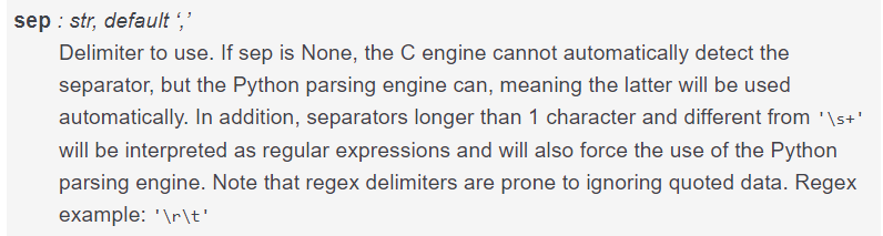
Hence, we can separate the columns by varying number spaces of spaces with sep='\s+' -parameter.
Our data also included No Data values with varying number of * -characters. Hence, we need to take also those
into account when reading the data. We can tell Pandas to consider those characters as NaNs by specifying na_values=['*', '**', '***', '****', '*****', '******'].
In [1]: data = pd.read_csv(fp, sep='\s+', na_values=['*', '**', '***', '****', '*****', '******'])
Exploring data and renaming columns
Let’s see how the data looks by printing the first five rows with head() function
In [2]: data.head()
Out[2]:
   index   USAF   WBAN  YR--MODAHRMN    DIR  SPD  GUS   CLG  SKC   L ...   \
0    216  29740  99999  201708040000  114.0  6.0  NaN   NaN  BKN NaN ...
1    217  29740  99999  201708040020  100.0  6.0  NaN  75.0  NaN NaN ...
2    218  29740  99999  201708040050  100.0  5.0  NaN  60.0  NaN NaN ...
3    219  29740  99999  201708040100  123.0  8.0  NaN  63.0  OVC NaN ...
4    220  29740  99999  201708040120  110.0  7.0  NaN  70.0  NaN NaN ...

      SLP    ALT    STP  MAX  MIN  PCP01  PCP06  PCP24  PCPXX   SD
0  1005.6    NaN  999.2  NaN  NaN    NaN    NaN    NaN    NaN  0.0
1     NaN  29.68    NaN  NaN  NaN    NaN    NaN    NaN    NaN  NaN
2     NaN  29.65    NaN  NaN  NaN    NaN    NaN    NaN    NaN  NaN
3  1004.7    NaN  998.4  NaN  NaN    NaN    NaN    NaN    NaN  0.0
4     NaN  29.65    NaN  NaN  NaN    NaN    NaN    NaN    NaN  NaN

[5 rows x 34 columns]
Let’s continue and check what columns do we have.
In [3]: data.columns
Out[3]:
Index(['index', 'USAF', 'WBAN', 'YR--MODAHRMN', 'DIR', 'SPD', 'GUS', 'CLG',
       'SKC', 'L', 'M', 'H', 'VSB', 'MW', 'MW.1', 'MW.2', 'MW.3', 'AW', 'AW.1',
       'AW.2', 'AW.3', 'W', 'TEMP', 'DEWP', 'SLP', 'ALT', 'STP', 'MAX', 'MIN',
       'PCP01', 'PCP06', 'PCP24', 'PCPXX', 'SD'],
      dtype='object')
Okey there are quite many columns and we are not interested to use all of them. Let’s select only columns that might be used to detect unexceptional weather conditions, i.e. YR–MODAHRMN, DIR, SPD, GUS, TEMP, MAX, and MIN.
In [4]: select_cols = ['YR--MODAHRMN', 'DIR', 'SPD', 'GUS','TEMP', 'MAX', 'MIN']

In [5]: data = data[select_cols]
Let’s see what our data looks like now by printing last 5 rows and the datatypes.
In [6]: data.tail()
Out[6]:
YR--MODAHRMN DIR SPD GUS TEMP MAX MIN
67 201708042220 180.0 11.0 NaN 61.0 NaN NaN
68 201708042250 190.0 8.0 NaN 59.0 NaN NaN
69 201708042300 200.0 9.0 11.0 60.0 NaN NaN
70 201708042320 190.0 8.0 NaN 59.0 NaN NaN
71 201708042350 190.0 8.0 NaN 59.0 NaN NaN
In [7]: data.dtypes
���������������������������������������������������������������������������������������������������������������������������������������������������������������������������������������������������������������������������������������������������������������������������������������������������������������������������������Out[7]:
YR--MODAHRMN int64
DIR float64
SPD float64
GUS float64
TEMP float64
MAX float64
MIN float64
dtype: object
The column names that we have are somewhat ackward. Let’s change them into more intuitive. This can be done easily with rename() -function.
We can define the new column names by using a specific data type in Python called dictionary where we can determine the original column name (the one which will be replaced), and the new column name.
Let’s change YR--MODAHRMN column into TIME, SPD into SPEED, and GUS into GUST
In [8]: name_conversion_dict = {'YR--MODAHRMN': 'TIME', 'SPD': 'SPEED', 'GUS': 'GUST'}
In [9]: print(name_conversion_dict)
{'YR--MODAHRMN': 'TIME', 'SPD': 'SPEED', 'GUS': 'GUST'}
In [10]: type(name_conversion_dict)
��������������������������������������������������������Out[10]: dict
Now we can change the column names by passing that dictionary into parameter columns in rename() -function.
In [11]: data = data.rename(columns=name_conversion_dict)

In [12]: data.columns
Out[12]: Index(['TIME', 'DIR', 'SPEED', 'GUST', 'TEMP', 'MAX', 'MIN'], dtype='object')
Perfect, now our column names are more easy to understand and use. Let’s check some basic statistics to understand our data better.
In [13]: data.describe()
Out[13]:
               TIME         DIR      SPEED       GUST       TEMP        MAX  \
count  7.200000e+01   72.000000  72.000000  20.000000  72.000000   2.000000
mean   2.017080e+11  229.555556  11.527778  17.700000  61.513889  66.500000
std    6.973834e+02  215.759248   3.756580   5.068998   3.175580   3.535534
min    2.017080e+11   80.000000   5.000000  11.000000  58.000000  64.000000
25%    2.017080e+11  117.750000   9.000000  13.000000  59.000000  65.250000
50%    2.017080e+11  200.000000  11.000000  16.000000  61.000000  66.500000
75%    2.017080e+11  220.000000  15.000000  22.250000  64.000000  67.750000
max    2.017080e+11  990.000000  20.000000  29.000000  69.000000  69.000000

             MIN
count   2.000000
mean   57.000000
std     1.414214
min    56.000000
25%    56.500000
50%    57.000000
75%    57.500000
max    58.000000
Okey so from here we can see that there are varying number of observations per column (see the count -information). For example SPD and TEMP column has 72 observations
whereas GUS has only 20 observations and MAX and MIN has only 2 observations.
From here we can already guess that MAX` and MIN attributes are most probably not going to be useful for us .
However, GUS might be.
Let’s explore further our data by checking the first 30 rows of it.
In [14]: data.head(30)
Out[14]:
            TIME    DIR  SPEED  GUST  TEMP   MAX   MIN
0   201708040000  114.0    6.0   NaN  58.0   NaN   NaN
1   201708040020  100.0    6.0   NaN  59.0   NaN   NaN
2   201708040050  100.0    5.0   NaN  59.0   NaN   NaN
3   201708040100  123.0    8.0   NaN  59.0   NaN   NaN
4   201708040120  110.0    7.0   NaN  59.0   NaN   NaN
5   201708040150  100.0    6.0   NaN  61.0   NaN   NaN
6   201708040200  138.0   10.0  13.0  59.0   NaN   NaN
7   201708040220  120.0   10.0   NaN  59.0   NaN   NaN
8   201708040250  100.0    9.0   NaN  59.0   NaN   NaN
9   201708040300  108.0    9.0  12.0  59.0   NaN   NaN
10  201708040320   90.0    8.0   NaN  59.0   NaN   NaN
11  201708040350   80.0    9.0   NaN  59.0   NaN   NaN
12  201708040400  102.0   11.0  15.0  58.0   NaN   NaN
13  201708040420   80.0   10.0   NaN  59.0   NaN   NaN
14  201708040450   80.0   10.0   NaN  59.0   NaN   NaN
15  201708040500  119.0   12.0  17.0  58.0   NaN   NaN
16  201708040520  990.0   11.0   NaN  59.0   NaN   NaN
17  201708040550  100.0   13.0   NaN  59.0   NaN   NaN
18  201708040600  121.0   16.0  23.0  58.0  64.0  56.0
19  201708040620  110.0   15.0   NaN  59.0   NaN   NaN
20  201708040650  100.0   15.0   NaN  59.0   NaN   NaN
21  201708040700  119.0   14.0  22.0  58.0   NaN   NaN
22  201708040720  990.0   14.0   NaN  59.0   NaN   NaN
23  201708040750  100.0   13.0   NaN  59.0   NaN   NaN
24  201708040800  125.0   10.0  15.0  58.0   NaN   NaN
25  201708040820  990.0    9.0   NaN  59.0   NaN   NaN
26  201708040850  100.0    7.0   NaN  59.0   NaN   NaN
27  201708040900  107.0    8.0   NaN  59.0   NaN   NaN
28  201708040920  990.0    7.0   NaN  59.0   NaN   NaN
29  201708040950  990.0    6.0   NaN  61.0   NaN   NaN
Okey, so from here we can actually see that the GUST column contains information only on an hourly level. That might be useful! Let’s keep this in mind.
Iterating rows and using self-made functions in Pandas
Let’s do the same thing as many times before and convert our Fahrenheit temperatures into Celsius. In this time, however, we will use our self-made function to do the conversion.
Here I provide you the function that you can copy and paste into your own script.
def fahrToCelsius(temp_fahrenheit):
    """
    Function to convert Fahrenheit temperature into Celsius.

    Parameters
    ----------

    temp_fahrenheit: int | float
        Input temperature in Fahrenheit (should be a number)
    """

    # Convert the Fahrenheit into Celsius and return it
    converted_temp = (temp_fahrenheit - 32) / 1.8
    return converted_temp
Let’s do the conversion by iterating our data line by line and updating a column called CELSIUS that we will create.
We can iterate over the rows of Pandas DataFrame by using iterrows() -function.
When iterating over the rows in our DataFrame it is noteworthy to understand that the Pandas actually keeps track on the index value as well.
Hence, the contents of a single row actually contains not only the values, but also the index of that row.
Let’s see how it works. Here, we will use a specific Python command called break can be used to stop the iteration right after the first loop.
This can be useful as we don’t want to fill our console by printing all the values and indices in our DataFrame, but to just see if the function works as we want.
In [15]: for idx, row in data.iterrows():
....: print('Index:', idx)
....: print(row)
....: break
....:
Index: 0
TIME 2.017080e+11
DIR 1.140000e+02
SPEED 6.000000e+00
GUST NaN
TEMP 5.800000e+01
MAX NaN
MIN NaN
Name: 0, dtype: float64
In [16]: type(row)
�������������������������������������������������������������������������������������������������������������������������������������������������������������������������������������������Out[16]: pandas.core.series.Series
Okey, so here we can see that the idx variable indeed contains the index value at position 0 (the first row) and the row variable contains all the data from that given row stored as a pd.Series.
Let’s now create an empty column for the Celsius temperatures and update the values into that column by using our function. Here is the whole procedure:
# Create an empty column for the data
col_name = 'Celsius'
data[col_name] = None

# Iterate ove rows
for idx, row in data.iterrows():
  # Convert the Fahrenheit temperature of the row into Celsius
  celsius = fahrToCelsius(row['TEMP'])
  # Add that value into 'Celsius' column using the index of the row
  data.loc[idx, col_name] = celsius
Let’s see what we have now.
In [17]: data.head()
Out[17]:
           TIME    DIR  SPEED  GUST  TEMP  MAX  MIN  Celsius
0  201708040000  114.0    6.0   NaN  58.0  NaN  NaN  14.4444
1  201708040020  100.0    6.0   NaN  59.0  NaN  NaN       15
2  201708040050  100.0    5.0   NaN  59.0  NaN  NaN       15
3  201708040100  123.0    8.0   NaN  59.0  NaN  NaN       15
4  201708040120  110.0    7.0   NaN  59.0  NaN  NaN       15
Great! Now we have converted our temperatures into Celsius by using the function that we created ourselves. Knowing how to use your own function in Pandas can be really useful when doing your own analyses. There is also another more powerful way of using functions in Pandas, see [1].
Let’s also convert the wind speeds into meters per second values (m/s) as they are more familiar to us in Finland. This can be done with a formula m/s = mph x 0.44704
In [18]: data['SPEED'] = data['SPEED']*0.44704

In [19]: data['GUST'] = data['GUST']*0.44704
Let’s see the result by printing the first 30 rows.
String manipulation in Pandas
In [20]: data.head(30)
Out[20]:
            TIME    DIR    SPEED      GUST  TEMP   MAX   MIN  Celsius
0   201708040000  114.0  2.68224       NaN  58.0   NaN   NaN  14.4444
1   201708040020  100.0  2.68224       NaN  59.0   NaN   NaN       15
2   201708040050  100.0  2.23520       NaN  59.0   NaN   NaN       15
3   201708040100  123.0  3.57632       NaN  59.0   NaN   NaN       15
4   201708040120  110.0  3.12928       NaN  59.0   NaN   NaN       15
5   201708040150  100.0  2.68224       NaN  61.0   NaN   NaN  16.1111
6   201708040200  138.0  4.47040   5.81152  59.0   NaN   NaN       15
7   201708040220  120.0  4.47040       NaN  59.0   NaN   NaN       15
8   201708040250  100.0  4.02336       NaN  59.0   NaN   NaN       15
9   201708040300  108.0  4.02336   5.36448  59.0   NaN   NaN       15
10  201708040320   90.0  3.57632       NaN  59.0   NaN   NaN       15
11  201708040350   80.0  4.02336       NaN  59.0   NaN   NaN       15
12  201708040400  102.0  4.91744   6.70560  58.0   NaN   NaN  14.4444
13  201708040420   80.0  4.47040       NaN  59.0   NaN   NaN       15
14  201708040450   80.0  4.47040       NaN  59.0   NaN   NaN       15
15  201708040500  119.0  5.36448   7.59968  58.0   NaN   NaN  14.4444
16  201708040520  990.0  4.91744       NaN  59.0   NaN   NaN       15
17  201708040550  100.0  5.81152       NaN  59.0   NaN   NaN       15
18  201708040600  121.0  7.15264  10.28192  58.0  64.0  56.0  14.4444
19  201708040620  110.0  6.70560       NaN  59.0   NaN   NaN       15
20  201708040650  100.0  6.70560       NaN  59.0   NaN   NaN       15
21  201708040700  119.0  6.25856   9.83488  58.0   NaN   NaN  14.4444
22  201708040720  990.0  6.25856       NaN  59.0   NaN   NaN       15
23  201708040750  100.0  5.81152       NaN  59.0   NaN   NaN       15
24  201708040800  125.0  4.47040   6.70560  58.0   NaN   NaN  14.4444
25  201708040820  990.0  4.02336       NaN  59.0   NaN   NaN       15
26  201708040850  100.0  3.12928       NaN  59.0   NaN   NaN       15
27  201708040900  107.0  3.57632       NaN  59.0   NaN   NaN       15
28  201708040920  990.0  3.12928       NaN  59.0   NaN   NaN       15
29  201708040950  990.0  2.68224       NaN  61.0   NaN   NaN  16.1111
When looking the data more carefully, we can see something interesting:
GUST seems to be measured only once an hour, whereas SPD (wind speed), and our temperatures seem to be measured approximately every 20 minutes (at minutes XX:00, XX:20 and XX:50).
That might be a problem as we might not be able to compare e.g. the average wind speeds and the speeds during the gust together as they are measured with different intervals. This kind of mismatch between sampling rates of measurements is actually quite typical when working with real data.
How we can solve this kind of problem is to aggregate the wind speeds into hourly level data as well so the attributes become comparable.
First we need to be able to group the values by hour. This can be done e.g. by slicing the date+hour time from the TIME column (i.e. removing the minutes from the end of the value)
- Doing this requires two steps:
- Convert the
TIMEcolumn fromintintostrdatatype. - Include only numbers up to hourly accuracy (exclude minutes) by slicing texts
- Convert the
Note
There are also more advanced functions in Pandas to do time series manipulations by utilizing datetime datatype and resample() -function, but we won’t cover those here. Read more information about creating datetime index and aggregating data by time with resampling from here if you are interested.
Let’s convert the time into string. And check that the data type changes.
In [21]: data['TIME_str'] = data['TIME'].astype(str)
In [22]: data.head()
Out[22]:
TIME DIR SPEED GUST TEMP MAX MIN Celsius TIME_str
0 201708040000 114.0 2.68224 NaN 58.0 NaN NaN 14.4444 201708040000
1 201708040020 100.0 2.68224 NaN 59.0 NaN NaN 15 201708040020
2 201708040050 100.0 2.23520 NaN 59.0 NaN NaN 15 201708040050
3 201708040100 123.0 3.57632 NaN 59.0 NaN NaN 15 201708040100
4 201708040120 110.0 3.12928 NaN 59.0 NaN NaN 15 201708040120
In [23]: data['TIME_str'].dtypes
����������������������������������������������������������������������������������������������������������������������������������������������������������������������������������������������������������������������������������������������������������������������������������������������������������������������������������������������������������������������������������������������������������������������������������������������������������������������������������������Out[23]: dtype('O')
In [24]: type(data.loc[0, 'TIME_str'])
������������������������������������������������������������������������������������������������������������������������������������������������������������������������������������������������������������������������������������������������������������������������������������������������������������������������������������������������������������������������������������������������������������������������������������������������������������������������������������������������������������Out[24]: str
Okey it seems that now we indeed have the TIME as str datatype as well.
Now we can slice them into hourly level by including only 10 first characters from the text (i.e. excluding the minute-level information).
In [25]: data['TIME_dh'] = data['TIME_str'].str.slice(start=0, stop=10)

In [26]: data.head()
Out[26]:
           TIME    DIR    SPEED  GUST  TEMP  MAX  MIN  Celsius      TIME_str  \
0  201708040000  114.0  2.68224   NaN  58.0  NaN  NaN  14.4444  201708040000
1  201708040020  100.0  2.68224   NaN  59.0  NaN  NaN       15  201708040020
2  201708040050  100.0  2.23520   NaN  59.0  NaN  NaN       15  201708040050
3  201708040100  123.0  3.57632   NaN  59.0  NaN  NaN       15  201708040100
4  201708040120  110.0  3.12928   NaN  59.0  NaN  NaN       15  201708040120

      TIME_dh
0  2017080400
1  2017080400
2  2017080400
3  2017080401
4  2017080401
Nice! Now we have information about time on an hourly basis including the date as well.
Note
Notice that all the typical str functionalities can be applied to Series of text data with syntax data['mySeries'].str.<functionToUse>().
Let’s also slice only the hour of the day (excluding information about the date) and convert it back to integer (we will be using this information later)
In [27]: data['TIME_h'] = data['TIME_str'].str.slice(start=8, stop=10)

In [28]: data['TIME_h'] = data['TIME_h'].astype(int)

In [29]: data.head()
Out[29]:
           TIME    DIR    SPEED  GUST  TEMP  MAX  MIN  Celsius      TIME_str  \
0  201708040000  114.0  2.68224   NaN  58.0  NaN  NaN  14.4444  201708040000
1  201708040020  100.0  2.68224   NaN  59.0  NaN  NaN       15  201708040020
2  201708040050  100.0  2.23520   NaN  59.0  NaN  NaN       15  201708040050
3  201708040100  123.0  3.57632   NaN  59.0  NaN  NaN       15  201708040100
4  201708040120  110.0  3.12928   NaN  59.0  NaN  NaN       15  201708040120

      TIME_dh  TIME_h
0  2017080400       0
1  2017080400       0
2  2017080400       0
3  2017080401       1
4  2017080401       1
Wunderbar, now we have also a separate column for only the hour of the day.
Aggregating data in Pandas by grouping
Next we want to calculate the average temperatures, wind speeds, etc. on an hourly basis to enable us to compare all of them to each other.
This can be done by aggregating the data, i.e.:
- grouping the data based on hourly values
- Iterating over those groups and calculating the average values of our attributes
- Inserting those values into a new DataFrame where we store the aggregated data
Let’s first create a new empty DataFrame where we will store our aggregated data
In [30]: aggr_data = pd.DataFrame()
Let’s then group our data based on TIME_h attribute that contains the information about the date + hour.
In [31]: grouped = data.groupby('TIME_dh')
Let’s see what we have now.
In [32]: type(grouped)
Out[32]: pandas.core.groupby.DataFrameGroupBy
In [33]: len(grouped)
����������������������������������������������Out[33]: 24
Okey, interesting. Now we have a new object with type DataFrameGroupBy. And it seems that we have 24 individual groups in our data, i.e. one group for each hour of the day.
Let’s see what we can do with this grouped -variable.
As you might have noticed earlier, the first hour in hour data is 2017080400 (midnight at 4th of August in 2017).
Let’s now see what we have on hour grouped variable e.g. on the first hour 2017080400.
We can get the values of that hour from DataFrameGroupBy -object with get_group() -function.
In [34]: time1 = '2017080400'

In [35]: group1 = grouped.get_group(time1)

In [36]: group1
Out[36]:
           TIME    DIR    SPEED  GUST  TEMP  MAX  MIN  Celsius      TIME_str  \
0  201708040000  114.0  2.68224   NaN  58.0  NaN  NaN  14.4444  201708040000
1  201708040020  100.0  2.68224   NaN  59.0  NaN  NaN       15  201708040020
2  201708040050  100.0  2.23520   NaN  59.0  NaN  NaN       15  201708040050

      TIME_dh  TIME_h
0  2017080400       0
1  2017080400       0
2  2017080400       0
Ahaa! As we can see, a single group contains a DataFrame with values only for that specific hour. This is really useful, because now we can calculate e.g. the average values for all weather measurements (+ hour) that we have (you can use any of the statistical functions that we have seen already, e.g. mean, std, min, max, median, etc.).
We can do that by using the mean() -function that we already used during the Lesson 5.
Let’s calculate the mean for following attributes: DIR, SPEED, GUST, TEMP, and Celsius.
In [37]: mean_cols = ['DIR', 'SPEED', 'GUST', 'TEMP', 'Celsius', 'TIME_h']

In [38]: mean_values = group1[mean_cols].mean()

In [39]: mean_values
Out[39]:
DIR        104.666667
SPEED        2.533227
GUST              NaN
TEMP        58.666667
Celsius     14.814815
TIME_h       0.000000
dtype: float64
Nice, now we have averaged our data and e.g. the mean Celsius temperature seems to be about right when comparing to the original values above. Notice that we still have information about the hour but not about the date which is at the moment stored in time1 variable.
We can insert that datetime-information into our mean_values Series so that we have the date information also associated with our data.
In [40]: mean_values['TIME_dh'] = time1

In [41]: mean_values
Out[41]:
DIR           104.667
SPEED         2.53323
GUST              NaN
TEMP          58.6667
Celsius       14.8148
TIME_h              0
TIME_dh    2017080400
dtype: object
Perfect! Now we have also time information there. The last thing to do is to add these mean values into our DataFrame that we created.
That can be done with append() -function in a quite similar manner as with Python lists.
In Pandas the data insertion is not done inplace (as when appending to Python lists) so we need to specify that we are updating the aggr_data (using the = sign)
We also need to specify that we ignore the index values of our original DataFrame (i.e. the indices of mean_values).
In [42]: aggr_data = aggr_data.append(mean_values, ignore_index=True)

In [43]: aggr_data
Out[43]:
     Celsius         DIR  GUST     SPEED       TEMP     TIME_dh  TIME_h
0  14.814815  104.666667   NaN  2.533227  58.666667  2017080400     0.0
Now we have a single row in our new DataFrame where we have aggregated the data based on hourly mean values.
Next we could continue doing and insert the average values from other hours in a similar manner but, of course, that is not
something that we want to do manually (would require repeating these same steps too many times).
Luckily, we can actually iterate over all the groups that we have in our data and do these steps using a for -loop.
When iterating over the groups in our DataFrameGroupBy object
it is important to understand that a single group in our DataFrameGroupBy actually contains not only the actual values, but also information about the key that was used to do the grouping.
Hence, when iterating over the data we need to assign the key and the values into separate variables.
Let’s see how we can iterate over the groups and print the key and the data from a single group (again using break to only see what is happening).
In [44]: for key, group in grouped:
   ....:     print(key)
   ....:     print(group)
   ....:     break
   ....:
2017080400
           TIME    DIR    SPEED  GUST  TEMP  MAX  MIN  Celsius      TIME_str  \
0  201708040000  114.0  2.68224   NaN  58.0  NaN  NaN  14.4444  201708040000
1  201708040020  100.0  2.68224   NaN  59.0  NaN  NaN       15  201708040020
2  201708040050  100.0  2.23520   NaN  59.0  NaN  NaN       15  201708040050

      TIME_dh  TIME_h
0  2017080400       0
1  2017080400       0
2  2017080400       0
Okey so from here we can see that the key contains the value 2017080400 that is the same
as the values in TIME_dh column. Meaning that we, indeed, grouped the values based on that column.
Let’s see how we can create a DataFrame where we calculate the mean values for all those weather attributes that we were interested in. I will repeate slightly the earlier steps so that you can see and better understand what is happening.
# Create an empty DataFrame for the aggregated values
aggr_data = pd.DataFrame()

# The columns that we want to aggregate
mean_cols = ['DIR', 'SPEED', 'GUST', 'TEMP', 'Celsius', 'TIME_h']

# Iterate over the groups
for key, group in grouped:
    # Aggregate the data
    mean_values = group[mean_cols].mean()

    # Add the ´key´ (i.e. the date+time information) into the aggregated values
    mean_values['TIME_dh'] = key

    # Append the aggregated values into the DataFrame
    aggr_data = aggr_data.append(mean_values, ignore_index=True)
Let’s see what we have now.
In [45]: aggr_data
Out[45]:
      Celsius         DIR      GUST     SPEED       TEMP     TIME_dh  TIME_h
0   14.814815  104.666667       NaN  2.533227  58.666667  2017080400     0.0
1   15.370370  111.000000       NaN  3.129280  59.666667  2017080401     1.0
2   15.000000  119.333333   5.81152  4.321387  59.000000  2017080402     2.0
3   15.000000   92.666667   5.36448  3.874347  59.000000  2017080403     3.0
4   14.814815   87.333333   6.70560  4.619413  58.666667  2017080404     4.0
5   14.814815  403.000000   7.59968  5.364480  58.666667  2017080405     5.0
6   14.814815  110.333333  10.28192  6.854613  58.666667  2017080406     6.0
7   14.814815  403.000000   9.83488  6.109547  58.666667  2017080407     7.0
8   14.814815  405.000000   6.70560  3.874347  58.666667  2017080408     8.0
9   15.370370  695.666667       NaN  3.129280  59.666667  2017080409     9.0
10  16.481481  225.000000   5.81152  4.768427  61.666667  2017080410    10.0
11  17.777778  241.666667   8.49376  5.513493  64.000000  2017080411    11.0
12  18.888889  228.333333   6.70560  5.960533  66.000000  2017080412    12.0
13  19.629630  229.666667   8.94080  7.152640  67.333333  2017080413    13.0
14  20.185185  228.666667  12.96416  8.940800  68.333333  2017080414    14.0
15  19.074074  218.333333  10.72896  7.450667  66.333333  2017080415    15.0
16  18.703704  214.666667  10.28192  7.152640  65.666667  2017080416    16.0
17  17.592593  209.666667   8.94080  7.003627  63.666667  2017080417    17.0
18  16.851852  211.333333  10.28192  5.662507  62.333333  2017080418    18.0
19  16.111111  203.000000   5.81152  4.023360  61.000000  2017080419    19.0
20  15.925926  198.000000   5.36448  4.023360  60.666667  2017080420    20.0
21  15.925926  186.666667       NaN  3.874347  60.666667  2017080421    21.0
22  15.555556  189.000000   6.70560  4.619413  60.000000  2017080422    22.0
23  15.185185  193.333333   4.91744  3.725333  59.333333  2017080423    23.0
Great! Now we have aggregated our data based on daily averages and we have a new DataFrame called aggr_data where all those aggregated values are stored.
Finding outliers from the data
Finally, we are ready to see and find out if there are any outliers in our data suggesting to have a storm (meaning strong winds in this case).
We define an outlier if the wind speed is 2 times the standard deviation higher than the average wind speed (column SPEED).
Let’s first find out what is the standard deviation and the mean of the Wind speed.
In [46]: std_wind = aggr_data['SPEED'].std()
In [47]: avg_wind = aggr_data['SPEED'].mean()
In [48]: print('Std:', std_wind)
Std: 1.6405694308360985
In [49]: print('Mean:', avg_wind)
������������������������Mean: 5.153377777777777
Okey, so the variance in the windspeed tend to be approximately 1.6 meters per second, and the wind speed is approximately 5.2 m/s. Hence, the threshold for a wind speed to be an outlier with our criteria is:
In [50]: upper_threshold = avg_wind + (std_wind*2)

In [51]: print('Upper threshold for outlier:', upper_threshold)
Upper threshold for outlier: 8.434516639449974
Let’s finally create a column called Outlier which we update with True value if the windspeed is an outlier and False if it is not.
We do this again by iterating over the rows.
# Create an empty column for outlier info
aggr_data['Outlier'] = None

# Iterate over rows
for idx, row in aggr_data.iterrows():
    # Update the 'Outlier' column with True if the wind speed is higher than our threshold value
    if row['SPEED'] > upper_threshold :
        aggr_data.loc[idx, 'Outlier'] = True
    else:
        aggr_data.loc[idx, 'Outlier'] = False
print(aggr_data)
Let’s see what we have now.
In [52]: print(aggr_data)
      Celsius         DIR      GUST     SPEED       TEMP     TIME_dh  TIME_h  \
0   14.814815  104.666667       NaN  2.533227  58.666667  2017080400     0.0
1   15.370370  111.000000       NaN  3.129280  59.666667  2017080401     1.0
2   15.000000  119.333333   5.81152  4.321387  59.000000  2017080402     2.0
3   15.000000   92.666667   5.36448  3.874347  59.000000  2017080403     3.0
4   14.814815   87.333333   6.70560  4.619413  58.666667  2017080404     4.0
5   14.814815  403.000000   7.59968  5.364480  58.666667  2017080405     5.0
6   14.814815  110.333333  10.28192  6.854613  58.666667  2017080406     6.0
7   14.814815  403.000000   9.83488  6.109547  58.666667  2017080407     7.0
8   14.814815  405.000000   6.70560  3.874347  58.666667  2017080408     8.0
9   15.370370  695.666667       NaN  3.129280  59.666667  2017080409     9.0
10  16.481481  225.000000   5.81152  4.768427  61.666667  2017080410    10.0
11  17.777778  241.666667   8.49376  5.513493  64.000000  2017080411    11.0
12  18.888889  228.333333   6.70560  5.960533  66.000000  2017080412    12.0
13  19.629630  229.666667   8.94080  7.152640  67.333333  2017080413    13.0
14  20.185185  228.666667  12.96416  8.940800  68.333333  2017080414    14.0
15  19.074074  218.333333  10.72896  7.450667  66.333333  2017080415    15.0
16  18.703704  214.666667  10.28192  7.152640  65.666667  2017080416    16.0
17  17.592593  209.666667   8.94080  7.003627  63.666667  2017080417    17.0
18  16.851852  211.333333  10.28192  5.662507  62.333333  2017080418    18.0
19  16.111111  203.000000   5.81152  4.023360  61.000000  2017080419    19.0
20  15.925926  198.000000   5.36448  4.023360  60.666667  2017080420    20.0
21  15.925926  186.666667       NaN  3.874347  60.666667  2017080421    21.0
22  15.555556  189.000000   6.70560  4.619413  60.000000  2017080422    22.0
23  15.185185  193.333333   4.91744  3.725333  59.333333  2017080423    23.0

   Outlier
0    False
1    False
2    False
3    False
4    False
5    False
6    False
7    False
8    False
9    False
10   False
11   False
12   False
13   False
14    True
15   False
16   False
17   False
18   False
19   False
20   False
21   False
22   False
23   False
Okey now we have at least many False values in our Outlier -column.
Let’s select the rows with potential storm and see if we have any potential storms in our data.
In [53]: storm = aggr_data.ix[aggr_data['Outlier'] == True]
In [54]: print(storm)
�������������������������������������������������������������������������������������������������������������������������������������������������������������������������������������������������������������������������������������������������������������������������������������������������������������������������������������������������������������������������������������������������������������������������������������������������������������������������������������������������������������������������������������������������������������������������������������������������������������������������������������������������������������������������������������������������������������������������������������������������������������������������������� Celsius DIR GUST SPEED TEMP TIME_dh TIME_h \
14 20.185185 228.666667 12.96416 8.9408 68.333333 2017080414 14.0
Outlier
14 True
Okey, so it seems that there was one outlier in our data but the wind during that time wasn’t that strong as the average speed was only 9 m/s. This is not too strange as we were only looking at data from a single day.
Repeating the data analysis with larger dataset
Let’s continue by executing the script that we have written this far and use it to explore outlier winds based on whole month of August 2017.
For this purpose you should change the input file to be 6591337447542dat_August.txt that you can download from here.
Note
Notice that if you haven’t written your codes into a script, you can take advantage of the History -tab in Spyder where the history of all your codes should be written from this session (you can copy / paste from there).
Change the input data for your script to be the whole month of August 2017 and run the same codes again.
After running the code again with more data, let’s see what were the mean and std wind speeds of our data.
In [55]: std_wind = aggr_data['SPEED'].std()
In [56]: avg_wind = aggr_data['SPEED'].mean()
In [57]: print('Std:', std_wind)
Std: 2.1405899770297245
In [58]: print('Mean:', avg_wind)
������������������������Mean: 4.1990832704402505
Okey so they are indeed different now as we have more data: e.g. the average wind speed was 5.2 m/s, whereas it is now only 4.2. Let’s see what we have now in our storm variable.
In [59]: storm
Out[59]:
       Celsius         DIR      GUST      SPEED       TEMP     TIME_dh  \
10   22.777778  210.666667  12.51712   9.089813  73.000000  2017080110
11   22.777778  212.000000  11.62304   8.940800  73.000000  2017080111
12   22.407407  205.666667  12.51712   9.089813  72.333333  2017080112
86   20.185185  228.666667  12.96416   8.940800  68.333333  2017080414
104  19.814815  204.333333  11.17600   8.791787  67.666667  2017080508
132  16.296296  237.666667  13.85824   9.387840  61.333333  2017080612
230  21.666667  217.000000  12.51712   8.642773  71.000000  2017081014
280  19.074074  700.666667  26.82240   8.791787  66.333333  2017081216
301  20.555556  210.000000       NaN   9.611360  69.000000  2017081313
302  19.444444  200.000000       NaN   8.493760  67.000000  2017081314
444  22.037037  195.666667  10.72896   8.493760  71.666667  2017081914
445  20.925926  204.666667  12.51712   8.940800  69.666667  2017081915
559  14.814815  328.666667  13.41120   8.493760  58.666667  2017082409
560  15.925926  329.333333  13.85824   8.493760  60.666667  2017082410
563  16.296296  329.666667  13.41120   9.238827  61.333333  2017082413
564  15.185185  550.000000       NaN   8.493760  59.333333  2017082414
686  17.222222  214.000000  13.41120   9.089813  63.000000  2017082916
687  17.037037  210.666667  11.62304   8.791787  62.666667  2017082917
704  18.518519  203.666667   8.04672   8.493760  65.333333  2017083010
705  18.888889  218.333333  13.41120   8.940800  66.000000  2017083011
706  17.962963  215.666667  14.52880  10.579947  64.333333  2017083012
707  17.962963  217.666667  12.07008   9.089813  64.333333  2017083013

     TIME_h Outlier
10     10.0    True
11     11.0    True
12     12.0    True
86     14.0    True
104     8.0    True
132    12.0    True
230    14.0    True
280    16.0    True
301    13.0    True
302    14.0    True
444    14.0    True
445    15.0    True
559     9.0    True
560    10.0    True
563    13.0    True
564    14.0    True
686    16.0    True
687    17.0    True
704    10.0    True
705    11.0    True
706    12.0    True
707    13.0    True
Okey, interesting! Now we can see the the days and hours when it has been stormy in August 2017.
It seems that the storms have usually been during the day time. Let’s check if this is the case.
We can easily count how many stormy observations for different hour of the day there has been by
using a value_counts() -function that calculates how many observations per certain value there are
in a certain column (works best for categorigal data).
Let’s see the counts for different hours of the day
In [60]: print(storm['TIME_h'].value_counts())
14.0    5
13.0    3
12.0    3
10.0    3
16.0    2
11.0    2
17.0    1
9.0     1
15.0    1
8.0     1
Name: TIME_h, dtype: int64
Okey, this is interesting. It seems that most often it has been stormy at 14:00 GMT (i.e. 16:00 at Finnish time). Notice, that there haven’t been any strong winds during the night, which is also interesting. However, as the The weather guys explains us, it is not that surprising actually =).
The average wind speed may not be the perfect measure to find extreme weather conditions. Gust might usually be a better measure for that purpose. Let’s see what were the strongest gust winds in our dataset by sorting the values.
In [61]: gust_sort = storm.sort_values(by='GUST', ascending=False)

In [62]: gust_sort
Out[62]:
       Celsius         DIR      GUST      SPEED       TEMP     TIME_dh  \
280  19.074074  700.666667  26.82240   8.791787  66.333333  2017081216
706  17.962963  215.666667  14.52880  10.579947  64.333333  2017083012
132  16.296296  237.666667  13.85824   9.387840  61.333333  2017080612
560  15.925926  329.333333  13.85824   8.493760  60.666667  2017082410
559  14.814815  328.666667  13.41120   8.493760  58.666667  2017082409
705  18.888889  218.333333  13.41120   8.940800  66.000000  2017083011
686  17.222222  214.000000  13.41120   9.089813  63.000000  2017082916
563  16.296296  329.666667  13.41120   9.238827  61.333333  2017082413
86   20.185185  228.666667  12.96416   8.940800  68.333333  2017080414
10   22.777778  210.666667  12.51712   9.089813  73.000000  2017080110
445  20.925926  204.666667  12.51712   8.940800  69.666667  2017081915
230  21.666667  217.000000  12.51712   8.642773  71.000000  2017081014
12   22.407407  205.666667  12.51712   9.089813  72.333333  2017080112
707  17.962963  217.666667  12.07008   9.089813  64.333333  2017083013
11   22.777778  212.000000  11.62304   8.940800  73.000000  2017080111
687  17.037037  210.666667  11.62304   8.791787  62.666667  2017082917
104  19.814815  204.333333  11.17600   8.791787  67.666667  2017080508
444  22.037037  195.666667  10.72896   8.493760  71.666667  2017081914
704  18.518519  203.666667   8.04672   8.493760  65.333333  2017083010
301  20.555556  210.000000       NaN   9.611360  69.000000  2017081313
302  19.444444  200.000000       NaN   8.493760  67.000000  2017081314
564  15.185185  550.000000       NaN   8.493760  59.333333  2017082414

     TIME_h Outlier
280    16.0    True
706    12.0    True
132    12.0    True
560    10.0    True
559     9.0    True
705    11.0    True
686    16.0    True
563    13.0    True
86     14.0    True
10     10.0    True
445    15.0    True
230    14.0    True
12     12.0    True
707    13.0    True
11     11.0    True
687    17.0    True
104     8.0    True
444    14.0    True
704    10.0    True
301    13.0    True
302    14.0    True
564    14.0    True
Interesting! There was one hour with quite extraordinary gust wind in our data happening at 12th of August in 2017. Indeed, that was a big storm in Helsinki called Kiira that caused major damage in different parts of the city.

Source: YLE Photo: Markku Sipi
| [1] | Below you can find information how to use functions in Pandas with an alternative way. |
Hint
Hint: Using iterrows() -function is not the most efficient way of using your self-made functions. In Pandas, there is a function called apply()
that takes advantage of the power of numpy when looping, and is hence much faster which can give a lot of speed benefit when you have millions of rows to iterate over.
Below I show how to do the similar thing by using our own function with apply().
I will make a copy of our original DataFrame so this does not affect our original data.
Before using this approach, we need to modify our function a bit to get things working.
First, we need to have a parameter called row that is used to pass the data from row into our function
(this is something specific to apply() -function in Pandas) and then add paramaters for passing the information about the column name that contains the temperatures in Fahrenheit,
and the column name where the coverted temperatures will be updated (i.e. the Celsius temperatures).
Hence, in the end, you can see that this is a bit more generic function to use (i.e. the columns to use in the calculation are not “hard-coded”).
def fahrToCelsius(row, src_col, target_col):
    """
    A generic function to convert Fahrenheit temperature into Celsius.

    Parameters
    ----------

    row: pd.Series
        Input row containing the data for specific index in the DataFrame

    src_col : str
        Name of the source column for the calculation. I.e. the name of the column where Fahrenheits are stored.

    target_col : str
        Name of the target column where Celsius will be stored.
    """
    # Convert the Fahrenheit into Celsius and update the target column value
    row[target_col] = (row[src_col]- 32) / 1.8
    return row
Take a copy of the data.
In [63]: data2 = data.copy()
Apply our new function and update the values into a new column called Celsius2
In [64]: data2 = data2.apply(fahrToCelsius, src_col='TEMP', target_col='Celsius2', axis=1)
As you can see here, we use the apply() function and as the first parameter
we pass the name of the function that we want to use with the apply(), and then we pass the names of the source column and the target column.
Lastly, it is important to add as a last parameter axis=1 that tells for the function to apply the calculations vertically (row by row) instead of horizontally (would move from column to another).
See the results.
In [65]: data2.head()
Out[65]:
           TIME    DIR    SPEED  GUST  TEMP  MAX  MIN    Celsius  \
0  201708040000  114.0  2.68224   NaN  58.0  NaN  NaN  14.444444
1  201708040020  100.0  2.68224   NaN  59.0  NaN  NaN  15.000000
2  201708040050  100.0  2.23520   NaN  59.0  NaN  NaN  15.000000
3  201708040100  123.0  3.57632   NaN  59.0  NaN  NaN  15.000000
4  201708040120  110.0  3.12928   NaN  59.0  NaN  NaN  15.000000

       TIME_str     TIME_dh  TIME_h   Celsius2
0  201708040000  2017080400       0  14.444444
1  201708040020  2017080400       0  15.000000
2  201708040050  2017080400       0  15.000000
3  201708040100  2017080401       1  15.000000
4  201708040120  2017080401       1  15.000000
Indeed it seems that our function worked because the values in Celsius and Celsius2 columns are the same.
With this approach it is extremely easy to reuse our function and pass the results into another new colum e.g.
In [66]: data2 = data2.apply(fahrToCelsius, src_col='TEMP', target_col='Celsius3', axis=1)

In [67]: data2.head()
Out[67]:
           TIME    DIR    SPEED  GUST  TEMP  MAX  MIN    Celsius  \
0  201708040000  114.0  2.68224   NaN  58.0  NaN  NaN  14.444444
1  201708040020  100.0  2.68224   NaN  59.0  NaN  NaN  15.000000
2  201708040050  100.0  2.23520   NaN  59.0  NaN  NaN  15.000000
3  201708040100  123.0  3.57632   NaN  59.0  NaN  NaN  15.000000
4  201708040120  110.0  3.12928   NaN  59.0  NaN  NaN  15.000000

       TIME_str     TIME_dh  TIME_h   Celsius2   Celsius3
0  201708040000  2017080400       0  14.444444  14.444444
1  201708040020  2017080400       0  15.000000  15.000000
2  201708040050  2017080400       0  15.000000  15.000000
3  201708040100  2017080401       1  15.000000  15.000000
4  201708040120  2017080401       1  15.000000  15.000000
Now we just added another column called Celsius3 just by changing the value of the target_col -parameter.
This is a good and efficient approach to use in many cases, and hence highly recommended (although it is a bit harder to understand).